Aug 9, 2026 OpenCV

OpenCV Python Contours and Matrices Practice: NumPy Matrix Operations + findContours Detailed Explanation

Introduction

In OpenCV Python, the essence of an image is a NumPy multi-dimensional array (also called a matrix or tensor). Whether it’s simple pixel assignment, channel separation, or complex contour detection and shape analysis, all operations are fundamentally matrix operations. Therefore, before diving deep into contour detection, mastering the basic operations of NumPy matrices is essential. This article will start from matrix basics and gradually transition to complete practice of cv2.findContours, helping you establish a complete cognitive chain from pixels to contours.

Part 1: NumPy Image Matrix Operations

The OpenCV version used in this example is: 4.1.1, running in Jupyter Notebook 6.0.0.

1. Load Dependencies

import cv2
import numpy as np
import matplotlib.pyplot as plt

2. Core Concepts of Matrices

Image matrices have two key characteristics - shape and data type (dtype):

shape: Dimension information of the matrix. For example, a 480×640 3-channel image has a shape of (480, 640, 3), representing height, width, and number of channels respectively.
dtype: Data type of each element in the matrix. np.uint8 means each element is an 8-bit unsigned integer, with a value range of 0～255.

3. Create Matrix Using np.full

# Create a 480x640 3-channel matrix, fill with 255 - get a pure white image
image = np.full((480, 640, 3), 255, np.uint8)

plt.figure(figsize=(9, 9))
plt.imshow(image)

Note: figsize defines the image window size in inches (1 inch = 2.54 cm), setting a larger value can make the image display more clearly.

4. Create Color Image by Specifying Channel Values

# Set third channel to 255, represents red in BGR mode
image = np.full((480, 640, 3), (0, 0, 255), np.uint8)

# matplotlib uses RGB color space, need to do BGR→RGB conversion first
image = cv2.cvtColor(image, cv2.COLOR_BGR2RGB)

plt.figure(figsize=(9, 9))
plt.imshow(image)

5. Fill Matrix Using fill

# Fill entire matrix with 0 - get a pure black image
image.fill(0)

plt.figure(figsize=(9, 9))
plt.imshow(image)

6. Specify Element Assignment - Single Point Operation

# Set pixels at three specified coordinates to white
image[240, 160] = image[240, 320] = image[240, 480] = (255, 255, 255)

plt.figure(figsize=(9, 9))
plt.imshow(image)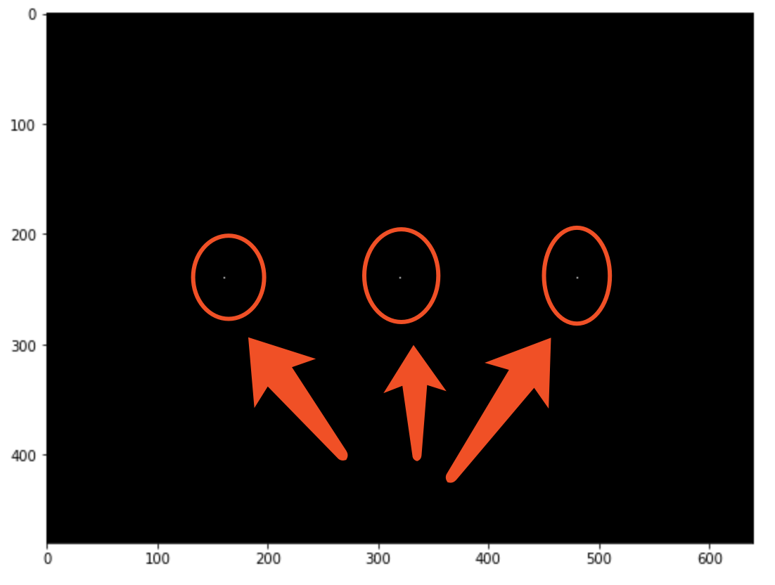

Looking carefully at the image, you can see 3 white pixel points, exactly located at the three coordinate positions [240, 160], [240, 320], [240, 480].

7. Specify Element Assignment - Entire Channel Operation

# Set first channel entirely to 255 (displays as red in RGB mode)
image[:, :, 0] = 255

plt.figure(figsize=(9, 9))
plt.imshow(image)

Note: Careful observation can still see the 3 white pixel points set earlier, because all three channels of them are already 255.

8. Specify Element Assignment - Vertical Line Operation

# Set all pixels on the middle vertical line of the image to white
image[:, 320, :] = 255

plt.figure(figsize=(9, 9))
plt.imshow(image)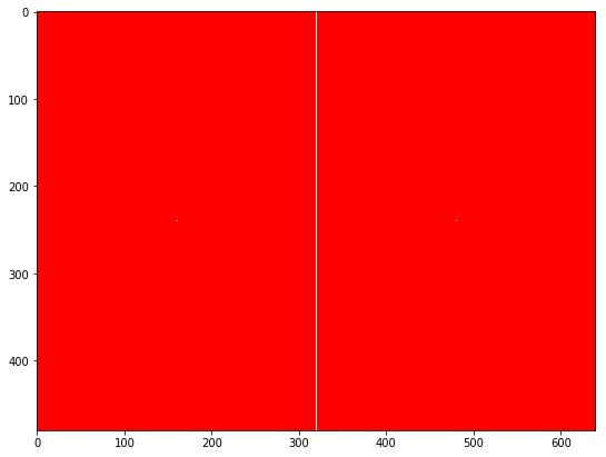

9. Specify Element Assignment - Region + Channel Operation

# In region [100:600, 100:200], set channel index 2 value to 255
# Channel index 2 is blue channel in RGB, red + blue = magenta
image[100:600, 100:200, 2] = 255

plt.figure(figsize=(9, 9))
plt.imshow(image)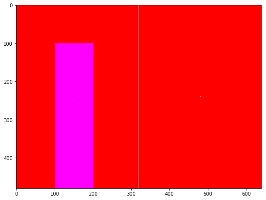

Matrix Operations Summary

Operation	Syntax	Description
Access element	`image[240, 160]`	Returns three-channel value array of that pixel
Access single channel	`image[240, 160, 1]`	Returns second channel value of that pixel
Full row/column selection	`image[:, 160]`	All pixels where y is 160
Region selection	`image[120:140, 160]`	Region where x is 120～140, y is 160
Entire channel assignment	`image[:, :, 0] = 255`	Set first channel entirely to 255

NumPy supports high-dimensional arrays and matrix operations, and also provides a large number of mathematical function libraries. When using deep learning frameworks like PyTorch, NumPy arrays can also be very conveniently converted to tensors for GPU processing.

Part 2: Contour Detection findContours

What is a Contour?

A contour can be simply explained as a curve connecting all consecutive points (along the boundary) that have the same color or intensity. Contours are a useful tool for shape analysis and object detection and recognition.

To obtain higher accuracy, using binary images works better. Therefore, before finding contours, please use thresholding or Canny edge detection first. Since OpenCV 3.2, findContours() no longer modifies the original image, so there’s no need to make a copy beforehand.

In OpenCV, finding contours is like finding white objects from a black background - the objects to be found should be white, and the background should be black.

Basic Usage

import numpy as np
import cv2 as cv

im = cv.imread('test.jpg')
imgray = cv.cvtColor(im, cv.COLOR_BGR2GRAY)
ret, thresh = cv.threshold(imgray, 127, 255, 0)
contours, hierarchy = cv.findContours(thresh, cv.RETR_TREE, cv.CHAIN_APPROX_SIMPLE)

The program first reads test.jpg, converts to grayscale, performs binarization with 127 as the threshold, then executes contour finding.

cv.findContours() has three parameters:

Source image: Input binary image.
Contour retrieval mode:
- RETR_EXTERNAL — Only retrieve outermost contours
- RETR_LIST — Retrieve all contours without establishing any hierarchical relationship
- RETR_CCOMP — Retrieve all contours and organize them into a two-level hierarchy. The top level is external boundaries of components, the second level is boundaries of holes
- RETR_TREE — Retrieve all contours and reconstruct the complete hierarchy of nested contours
- RETR_FLOODFILL — Connected components of multi-level images
Contour approximation method (see below for details).

Return value contours is a Python list, each element is a NumPy array of (x, y) coordinates of object boundary points. hierarchy describes the nesting relationship between contours.

Draw Contours

Use cv.drawContours() function to draw contours:

# Draw all contours
cv.drawContours(img, contours, -1, (0, 255, 0), 3)

# Draw 4th contour
cv.drawContours(img, contours, 3, (0, 255, 0), 3)

# More common approach: extract contour first then draw
cnt = contours[4]
cv.drawContours(img, [cnt], 0, (0, 255, 0), 3)

Contour Approximation Methods

This is the third parameter of cv.findContours, determining whether contours store all boundary points:

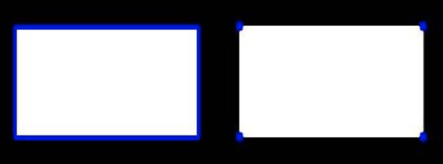
cv.CHAIN_APPROX_NONE: Stores all boundary points.
cv.CHAIN_APPROX_SIMPLE: Removes redundant points and compresses contours, saving memory. For example, a straight line only needs to keep two endpoints.

The rectangular image below intuitively demonstrates the difference: CHAIN_APPROX_NONE gets 734 points, while CHAIN_APPROX_SIMPLE only gets 4 points - the memory saving effect is very significant!

Practical Comparison of Different Thresholds

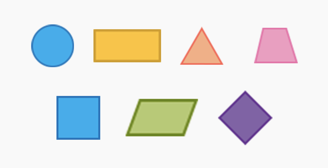
Let’s take an image containing various shapes as an example to compare contour detection effects under different threshold parameters.

Original image:

Parameters: threshold=127, contour retrieval mode=RETR_TREE, contour approximation method=CHAIN_APPROX_SIMPLE

Original	After Grayscale	After Threshold	Draw Contours

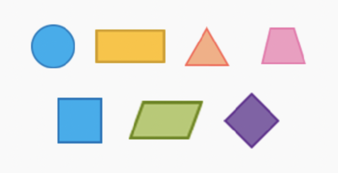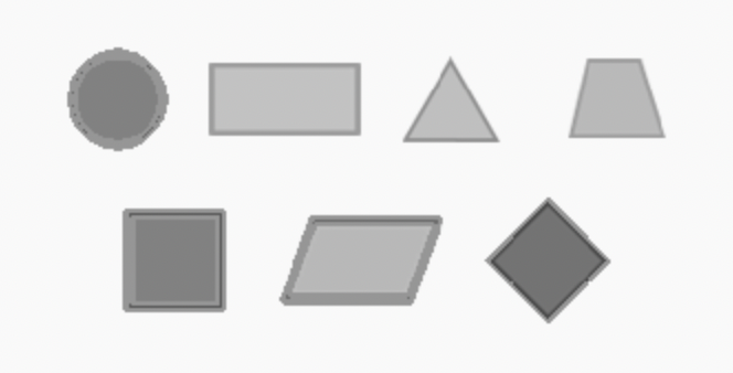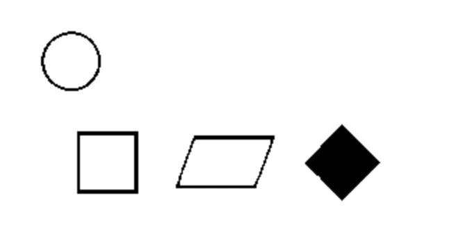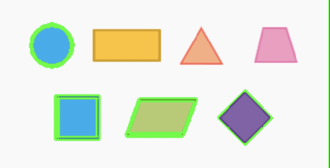From the processing results, we can see that because the threshold is too low, warm-colored shapes are filtered out, unable to correctly obtain all contours.

Parameters: threshold=200, contour retrieval mode=RETR_TREE, contour approximation method=CHAIN_APPROX_SIMPLE

Original	After Grayscale	After Threshold	Draw Contours

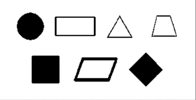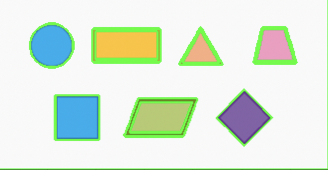Although this time all contours are drawn, another problem is also found: the edges of the entire image and inner circles of some shapes are also drawn with contours.

As for the sequential relationship between these contours, we will discuss it in detail in subsequent articles.

Part 3: Matrix + Contour Comprehensive Practice

After understanding matrix operations and contour detection, we can combine the two: use NumPy to create image matrices and draw shapes, then use findContours to detect the contours of these shapes.

import numpy as np
import cv2 as cv
import matplotlib.pyplot as plt

# 1. Use NumPy to create a black background image
image = np.full((480, 640, 3), 0, np.uint8)

# 2. Draw white shapes on the matrix
cv.rectangle(image, (50, 50), (200, 200), (255, 255, 255), -1)    # White rectangle
cv.circle(image, (400, 240), 100, (255, 255, 255), -1)             # White circle
cv.line(image, (250, 400), (550, 400), (255, 255, 255), 3)         # White line

# 3. Convert to grayscale + threshold processing
gray = cv.cvtColor(image, cv.COLOR_BGR2GRAY)
ret, thresh = cv.threshold(gray, 127, 255, 0)

# 4. Find and draw contours
contours, hierarchy = cv.findContours(thresh, cv.RETR_TREE, cv.CHAIN_APPROX_SIMPLE)
cv.drawContours(image, contours, -1, (0, 255, 0), 2)

# 5. Display results
plt.figure(figsize=(9, 9))
plt.imshow(cv2.cvtColor(image, cv.COLOR_BGR2RGB))
plt.title(f'Detected {len(contours)} contours')
plt.show()

This code completely demonstrates the workflow: create matrix → draw shapes → grayscale conversion → threshold processing → contour detection → result visualization. Through matrix operations, you can precisely control every pixel in the image, while contour detection allows you to rise from pixel-level to shape-level analysis and understanding.

Summary

Matrix operations are the cornerstone of OpenCV image processing - from creating blank canvases to precise pixel-level editing, NumPy provides powerful and flexible toolchains. Contour detection is the core entry point for shape analysis and object recognition, cv2.findContours can adapt to various scenarios from simple geometry to complex nested structures through different retrieval modes and approximation methods. Mastering these two parts of knowledge, you have complete image processing capabilities from low-level pixels to high-level semantics.